Basic Overview¶

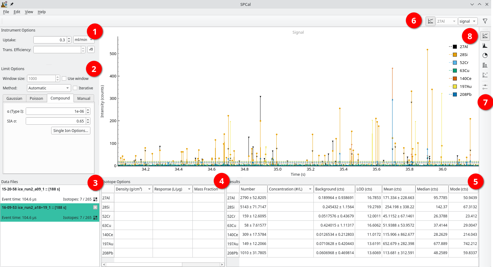
../_images/usage_overview.png — Fig. 5 The main SPCal window with a TOF data file loaded. ① Instrument specific options. ② Limit (thresholding) options. ③ Currently loaded data files. ④ Isotope specific options. ⑤ Results summary. ⑥ The main toolbar. ⑦ The view toolbar. ⑧ The main view, showing particle data.¶

The SPCal GUI consists of a main window where data is plotted (Fig. 5 ⑧) with several moveable docks (Fig. 5 ① to ⑤) and two toolbars (Fig. 5 ⑥ and ⑦). Docks can be reorganised or hidden to make a layout thats suits you. This layout is saved on exit and restored when SPCal starts. To restore hidden docks use View -> Show/hide dock widgets and to restore the default layout View -> Restore Default Layout.

Descriptions of each dock can be found below.

Instrument Options¶

This dock displays instrument specific options that are used during calibration of signals to masses and sizes. The Uptake is the sample uptake, in the displayed units. The Trans. Efficiency is the transport efficiency, a value between 0 and 1 that represents the fraction of particles in a sample that reach the plasma. See Calibration for more information. To calculate the transport efficiency use the button next to Trans. Efficiency. This button is active once particles are detected and the uptake is specified.

Limit Options¶

A dock containing options specific to the thresholding of data. See Thresholding Options for details on each method and Thresholds for spICP-MS for background and theory.

Data Files¶

A list of data files currently loaded into SPCal, with their names, total length in seconds, event time and isotopes. Files can be closed using the button in the top right and isotopes (re)selected using the button in the bottom left. Right-clicking the file will open a context menu allowing access to the isotope selection and additional information.

Selecting multiple files (with Shift) will cause all selected files to be plot in the main view (Fig. 5 ⑧).

Isotope Options¶

This dock displays options specific to individial isotopes. The density can be selected using the Density Database by right-clicking the density field. Similarly, the mass fraction can be selected using the Mass Fraction Calculator by right-clicking the mass fraction field. The mass fraction can also be calculated by inputing the molecular formula directly into the field, with the isotope of interest first (e.g., as FeO3 for the iron fraction or as O3Fe for the oxygen fraction).

While a method may contain more isotope options, only isotopes selected for the current file are displayed here.

Results¶

A summary of the particle detection results for the selected data file. By changing the Key in the Main Toolbar (Fig. 5 ⑥) the particle results can be display in Signal, Mass or Size. Values for isotopes that cannot be calibrated to the required Key will be left blank. The display units can be changed by left-clicking the header.

Right-clicking the isotope labels on the left will open a context menu with new options. Here, you can remove an isotope or isotope expression or easily sum the selected isotopes.

Main View Area¶

Here data and results are displayed. The specific view can be selected using the View Toolbar.