Thresholds for spICP-MS
Poisson
At the very low counting rates often seen in spICP-MS work, the typical Gaussian statistics (\(\mu + 3 \sigma\)) used to determine detection limits do not apply. Instead Poisson statistics should be used to determine the critical value, the threshold above which a signal is considered to be a detected particle [1] . Confusingly, most Poisson statistics will also define a detection threshold, but this should not be used to determine the detection of signal. There are a number of different (more or less permissive) formulas for determining these thresholds, most of which are implemented in SPCal. In general, the Currie method with an ε value of 0.5 works well and is recommended.
spICP-ToF: Compound-Poisson
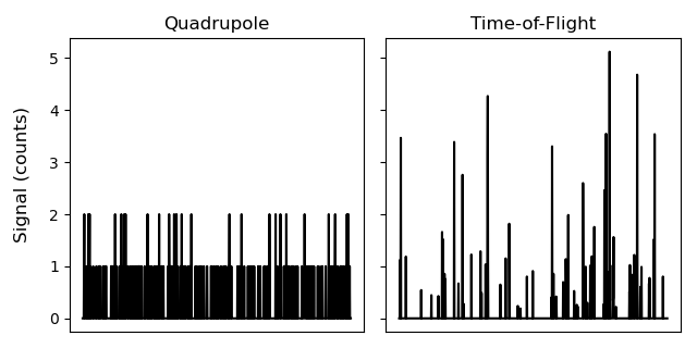
Fig. 1 The data produced by a ToF MS is non-integer.
The Poisson thresholding typically used for spICP-MS is not valid for spICP-ToF, as is easily established by looking at spICP-ToF data. Unlike data from a quadrupole instrument, this data is non-integer. To achieve sufficient resolution a time-of-flight instrument cannot be operated in pulse-counting mode, where the electron pulses from individual ions are counted as discrete (integer) events [2] . Instead, the detectors in TOFs use the raw output of fast analogue-to-digital converters and this exposes the variation in current produced by an electron multiplier for a single ion, known as the pulse-height distribution (PHD) or single ion area (SIA) [3] . The result of multiple ions striking the detector is therefore a Poisson sampling of the PHD, where each ion may produce a range of values.
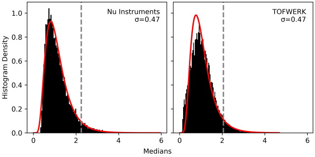
Fig. 2 The single ion area of two ICP-ToF instruments, and log-normal fits.
To convert these values into counts the detector is calibrated to determine the SIA, typically by analysing a very low concentration sample, i.e. one that is likely to only produce single-ion events. Multiple acquisitions of raw data from the detector are summed and then normalised to approximate the signal produced for 1 ion (count) by dividing by the mean of the recorded SIA.
Compound-Poisson sampling must be used to accurately determine a detection threshold for spICP-ToF, ideally of the actual SIA of the instrument [3] . In SPCal, this can be performed by brute force simulation or by using a log-normal approximation of the SIA. For both methods, the lambda (mean) value of the Poisson is taken as the mean signal in the data set. The simulation uses a given SIA distribution to generate a compound-Poisson distributed data and determines the threshold from the appropriate quantile of this data. While accurate at high error rate (\(>10^{-3}\)) the computational cost to simulate enough samples for low error rate is too high to be practical [4] .
Log-normal approximation
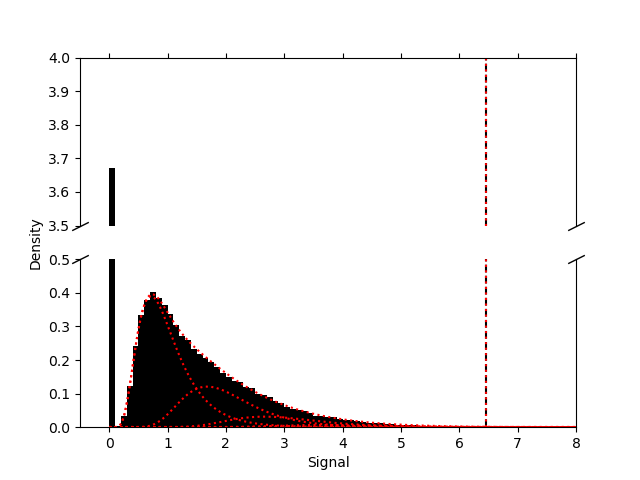
Fig. 3 A spICP-ToF background and the corresponding log-normal approximation. Each log-normal (red) is summed to estimate the non-zero portion of the compound-Poisson distributed data.
The log-normal approximation works by closely approximating the SIA with a log-normal distribution, see Fig. 2. Since the cumulative density and quantile functions of a log-normal are known, we can then predict the resulting detection threshold for the sum of log-normal distributions. In the case of the log-normal approximation only the shape parameter (\(\sigma\)) of the log-normal fit to the SIA is required.
Warning
The log-normal approximation method is depreciated and no longer used in spcal versions 2.0.0 and above.f
Lookup Table
Similar to the Log-normal approximation the lookup table assumes the SIA can be approximated using a log-normal distribution. The lookup table is a 3-dimensional array of quantiles calculated for a zero-truncated compound-Poisson-log-normal distribution. Each quantile comes from a simulation of \(10^{10}\) values using the parameters in the table below, using the computational facilities of the UTS eResearch High Performance Computer Cluster. Values between simulated points are interpolated at a sub 0.2 % error.
Parameter |
Range |
No. Values |
|---|---|---|
\(\lambda\) |
0.001 - 100 (geometric) |
71 |
\(\sigma\) |
0.25 – 0.95 (linear) |
41 |
\(\alpha\) (zero-truncated) |
0.999 – \(10^{-7}\) (logistic) |
101 |
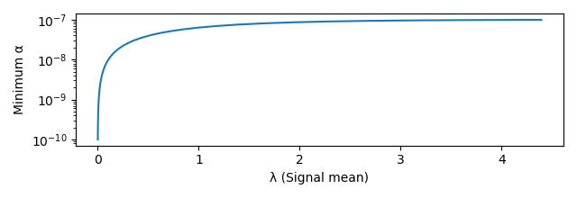
Fig. 4 The minimum valid alpha value (α) varies with the signal mean (λ). As λ decreases, the number of zero values increases and thus the zero-truncated α value used in the lookup table will represent a smaller (non-zero-truncated) Compound-Poisson α.
Threshold selection
Number of non-zero values below 5 counts |
Number of non-zero values \(\mathbb{Z} \pm 0.05\) |
Threshold method |
|---|---|---|
\(>5%\) |
Gaussian |
|
\(<5%\) |
\(>75%\) |
Poissson |
\(<5%\) |
\(<75%\) |
compound-Poisson |
The best method to find the detection threshold will depend on the data being analysed. SPCal will use aspects of the loaded sample to choose between using Gaussian, Poisson of compound-Poisson statistics. For data that is consistently above five counts, Gaussian statistics are used, otherwise Poisson or compound-Poisson depending on the integer nature of the data. Values are considered integer if they are within 0.05 of an integer value, as data exports from ICP-MS often seem to have a small offset from true integers. The detection threshold is then calculated for the chosen error rate (\(\alpha\)).
Error rates
In other analytical techniques a 5% error rate (\(\alpha = 0.05\)) is considered acceptable and is frequently used implemented as the \(3 \sigma\) rule. However, the large number of events collected during spICP-MS makes such low error rate lead to a very large number of false detections. An error rate of \(\alpha = 10^{-6}\) is fairly standard and will lead to only 1 false detection per million events.